OR 568: Applied Predictive Analytics

Final Report

Ames Housing Dataset: Predicting the House Sale Price

Data Panthers: Aakriti Garg, Chu Chuan Jeng, Ganesh Nalluru, Kalkidan Ashenafi, Sai

Hemanth Nirujogi, Siva Swetha Yalamanchili

Abstract

The price of a house can’t be predicted by studying the number of bedrooms and bathrooms, the height of the ceiling, the age of the property or even the extensive study of the neighborhood. A house that becomes a home of a family needs to tick off all the boxes. A house buyer considers a lot more than the statistics of the property before investing his/her hard earned money into it.

This project attempts to expand the house prediction model to predict the sale price of a house in Ames, Iowa by taking into account various parameters a house buyer is most likely to consider. We are using the Ames housing dataset that consists of 79 explanatory variables i.e, 37 quantitative and 42 qualitative that describe almost every possible aspect of residential homes.

Objectives

The objective of this project is to identify the features that are the best predictors of the sale price of the houses and to predict the sale price of each house in the dataset. Therefore, we can answer the driven question: How much will a house sell for in Ames, Iowa?

Data

Data Description

The Ames Housing dataset was compiled by Dean De Cock for use in data science education. This dataset is believed to be a modernized and expanded alternative of the Boston Housing dataset. We were able to download this dataset from Kaggle.com (Cock, 2011). There are two primary datasets train.csv and test.csv. The training data (train.csv) has 1460 data points and total variable count of 81, with an ID column, 79 explanatory variables, one response variable i.e., SalePrice. And, the test data (test.csv) has 1459 data points and total variable count of 81, with an ID column, 79 explanatory variables.

Data Type

The dataset used contains 79 explanatory variables and these variables are a combination of quantitative and qualitative variables. We need to understand the variable type and measurement scale of each of the predictor to employ the right visualization for exploratory analysis. This also helps us perform suitable statistical techniques to impute the missing values and finally to choose the right data analysis model for the selected predictors.

Data Preparation

The data from Kaggle was in a raw format and needed cleaning. Also, we knew with a large number of variables in the dataset, we needed to process the data before we could use it for developing the predictive model.

We combined the test and training data provided by Kaggle and started with analyzing the data for missing values, as a starting point we decide to concentrate on the variables that had more 90% of the data missing and/or had none values. We found five variables that either had 90% of the data or had a not available (or none) for that variable. These variables were identified are the variables for the Pool Area, Pool Quality, Fence Type, Alley Type, Fireplace Quality (Figure 1).

Figure 1. Understanding Missing Data

To decide the right course of action for these variables, we compared the average sale price with and without these variables. Except for variables for the pool, we found that the average sale price of the house was same with and without the average, for instance, the average sale price of the house with a fence or without a fence was very similar. Hence we decided to drop these variables. While comparing the variables for the pool we observed that the average sale price of a house with pool was $1million higher than the house that did not have a pool (Figure 2). While we understand it will be ideal to develop two separate data model for the house with and without the pool, we were unable to do so due to the lack of data for the houses with pool.

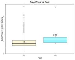
Figure 2. Compared the Variables for the Pool

Next, we looked for were the outliers in the data and found that there were a couple of houses with square feet area greater than two standard deviations of the average square feet are. We decide to delete outlier from the dataset. We then looked for a correlation between variables and removed the highly correlated variables (Figure 3). Then the imputation techniques were performed of the remaining missing data. The missing values for numerical variables were replaced by the mean values and the missing values for the categorical variables are replaced by the most frequently occurring or the mode values.

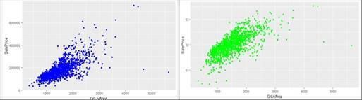
Figure 3. Correlation Plot of SalePrice vs GriLiveArea (Blue is original, & Green is after cleaning)

The data has been preprocessed using the function preProcess() for the center, scale and Box-cox, additionally the variables with near zero variance are removed. To convert character columns to factors, dummy variables were then created for categorical variables. The response variable, SalePrice was right skewed and hence log-transformation was applied. Hence, for our final predictions, we are taking the exponential on the predicted values (Figure 4).

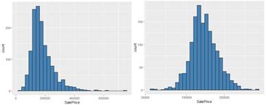
Figure 4. Box-Cox Log-transformation on the Response Variable

Finally, the data after the preprocessing has 267 numerical values and no categorical values as they have been converted into numerical values as well, so that regression models could be developed on the data. The data was then again split to train and test data and the original data count of the dataset was maintained.

Exploratory Data Analysis

Exploratory data analysis were performed to get insights from the data about the trends and patterns we can observe from the data without performing any data modeling techniques. The data exploration helped us understand the dataset and what we could expect from the data, while also helping us evaluate the quality of data. In our approach for the project, we choose to use data exploration as an iterative step, as we relied heavily on data exploration to validated our approach to data clean and even our findings.

The following are five interesting insights we gained data exploration:

● The average sale price of a house with a swimming pool is over a million dollars higher than the average sale price of a house with no swimming pool (Figure 2).

● A house with a newer architecture has higher sale price (Figure 5).

● We observed that some house that was built before the 19th century were higher than the houses built between the year 1940 to 1980. We believe this could be the house that has a vintage value (Figure 5).

● As expected the sale price of the house has been increasing with years passing, but we see that the house price was the highest around the year 2007 (Figure 6).

● There is a sudden dip in the sale price of the house in the year 2008, a house that was sold for over $7million in the year 2007 was sold for $4million in the year 2008. And we believe this could be due to the recession that hit (Figure 6).

Figure 5. The trend of Sale Price vs Year Built Figure 6. The trend of Sale Price vs Year Sold

Feature Engineering Data Models 1. Principal Component Analysis (PCA)

After cleaning the outliers, missing values, and inconsistent data, we need to check if there is any multicollinearity for the numerical predictors. It is very important to prepare the data for further analysis. Principal Components Analysis (PCA) is an unsupervised learning method that could reduce the dimension efficiently avoiding the multicollinearity.

According to the result of the PCA, Importance of the components (Table 1), the cumulative proportion of the first components could explain up to 95% and the second component can explain nearly 97%. Hence, the result of the cumulative proportion of the components that reach 99% is meaningless. Therefore, using the first component only or the first and second components could explain the predictors in this case.

	Comp.1	Comp.2	Comp.3	Comp.4	Comp.5	Comp.6	Comp.7	Comp.8	Comp.9	Comp.10
Standard deviation	215.10	35.27	32.68	15.20	3.79	3.79	3.16	2.72	2.45	2.41
Proportion of Variance	0.94	0.04	0.02	0.00	0.00	0.00	0.00	0.00	0.00	0.00
Cumulative Proportion	0.94	0.97	0.99	0.10	0.10	0.10	0.10	0.10	0.10	010

Finally, there are 14 predictors in total extracted based on the corresponding eigenvalue (estimate the proportion of total variability of variables by the principal components) which are higher than 30% in component 1 and 2 summarized in Table 2. These 14 predictors could help us do the further predictive modeling.

Comp.1	SalePrice	OverallQual	GrLivArea	GarageArea	FullBath	TotalBsmtSF
	1stFlrSF	YearBuilt	YearRemodAdd
Comp.2	2ndFlrSF	BedroomAbvGr	ToRmAbvGrd	BsmtFinSF1	GrLivArea	HalfBath

Table 2. Important Predictors Selected by the eigenvalue over 30%

2. Ridge & Lasso Regression Models

An extra component in Ridge regression is L2 penalty term which is given as λ (lambda) and the sum of Beta squares. While minimizing the sum of squared errors using ridge regression the L2 penalty term shrinks coefficients. For Lasso regression, the sum of squares due to error, we have λ multiplied with the sum of absolute value of Beta, L1 penalty term. This L1 penalty term shrinks coefficients to zero and the shrinking of coefficients to zero is useful for feature selection.

We have tuned our parameter by setting a sequence to create a series. For ridge regression, we set our alpha to zero and create a sequence for λ starting with a number that is close to zero to one. λ is a hyperparameter and it's estimated using cross-validation that we specified using our custom train control and its the strength of the penalty on the coefficients. Figure 8 and Figure 9 are for Ridge and Lasso regression models produce. Both plots show that increasing lambda increases RMSE, from Ridge regression the most optimal λ= 0.0001.

Figure 8. Ridge Regression Model Result Figure 9. Lasso Regression Model Result

3. Multivariate Adaptive Regression Splines (MARS)

The data does not show the linear relationship and needed a model that is robust to departure for linearity. Hence, we chose to develop a MARS model as we know that MARS uses surrogate features instead of the original predictors to extend the linear model to capture non-linear relationships. MARS creates two contrasted versions of a predictor to enter the model and these surrogate features in MARS are usually a function of only one or two predictors at a time. The algorithm of the MARS is to break the predictor into two groups to create a piecewise linear model capturing the linear relationships between the predictor and the outcome in each group. For the cut point for a predictor, two new features are hinge or hockey stick functions of the original predictor. The new features are added to a basic linear regression model to estimate the slopes and intercepts.

There are two tuning parameters associated with the MARS model: the degree of the features that are added to the model and the number of retained terms (i.e., nprune). The MARS helps feature selection, as it selects the predictor that helped create the optimal number of terms that were enough to capture the linear relationship from a non-linear data.

For the MARS developed for the data, we first used an internal GCV technique to get an estimate of the tuning parameters. We found that degree = 1 and nprune = 28 would be an optimal combination.

Then we performed a grid search to identify the optimal combination of these tuning parameters. We found the values of tuning parameter, degree = 1 and nprune = 29 is the most optimal value for our model.

Figure 10.GRsq vs No. of Items Figure 11.RMSE vs Terms

4. Support Vector Machines

Support vector machines are one of the powerful and flexible modeling tools. As our data is non-linear, we use the radial basis function for effective results. Cost parameter is one of the essential tuning parameters for SVM. Increase in the cost value makes the model flexible and amplifies the errors. With low-cost values, the model tends to over-fit (Kuhn & Johnson, 2013).

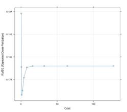
Figure 12. SVM RMSE vs Cost

Figure 12 shows the RMSE values against cost values. We can observe that RMSE value is minimum for Cost =1. Model tuning is done using tune() to find the best tuning parameters and these values are plugged into the model and tuned again to obtain better results (Kuhn & Johnson, 2013).

KNN Model

The K -nearest neighbor is a supervised learning algorithm which uses the entire dataset in its training phase. We are using KNN to predict the unseen data and the data with the most similar instances in our dataset. The model is trained on our dataset to find the most common classification of these entries. From the graph (Fig.13), we can see that the least RMSE value is achieved at K=9. The RMSE value of the KNN model is very high compared to the other models used in this project.

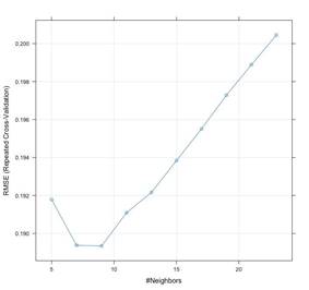
Fig.13 KNN - RMSE vs K Neighbors

Feature Selection

We would expect the sale price of the house to be driven by three main factors, the square footage

(or the area) of the house, the condition of the house and the neighborhood of the house. We used PCA, random forest, LASSO and MARS to perform feature selection, to help us understand what the top predictors that influence the sale price of the house.

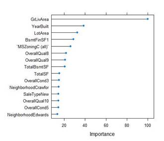
Figure 14. Variable Importance from MARS

The following are three observations from the findings of our feature selection techniques:

● The neighborhoodDiagramot appears to be amongst the top 10 predictors for all of the models developed for feature selection.

● Total above the ground area of the house did appear to be among the top predictors three of the sale price.

● Similarly, as expected the overall quality of the house did appear to be among the top predictors three of the sale price.

Our further analysis of the neighborhood shows while there is a variable in the average sale price between the different neighborhoods (Figure 15), the variation in the average price isn’t as much as we would typically expect. The variation is observed only between the outliers, and while that does influence the average, the average doesn’t show much variation and we believe that if their outlier were not present the average price between the house from the different neighborhood would have been very more close. Also, two neighborhoods that do show some influence on the sale price is the neighborhood with the lower average sale price and one with the average value of the average sale price.

Figure 15. Box Plot of Sale Price vs Neighborhoods

Results/Findings

Summary of results from all the models:

		TRAINING RESULTS
	RMSE	R-squared	SDRMSE	R-Square SD
Ridge Regression	0.0964	0.9421	0.0116	0.0167
LASSO Regression	0.0894	0.9495	0.0108	0.0165
Elastic Net Regression	0.0918	0.9469	0.0117	0.0168
KNN	0.1893	0.7895	0.0189	0.0309
Linear Regression after PCA	0.3013	0.4319	0.0165	0.0583
MARS	0.1168	0.9279	0.0145	0.0204
SVM	0.1766	0.8057	0.0304	0.0553

Table 3. Summary of the models

Kaggle results:

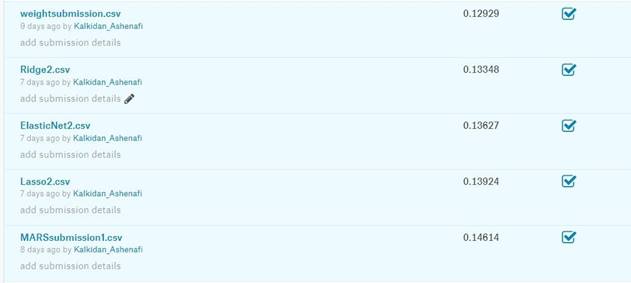
Fig.16 Results on the test dataset from Kaggle

Conclusion

From the results obtained for the data models, we can see that the Ridge model has the least RMSE value and hence it the optimal to predict best housing price. Lasso, Elastic net also have the next best results while computed on the test dataset. We can also the infer from the results that SVM, KNN models are not recommendable for this particular data set.

Most Important Predictors:

The most Important predictors are GrLivArea,YearBuilt, and LotArea and we agree that they are important.

Step by Step instructions on how to run the code

Step1: Open the

“Ashenafi_Garg_Jeng_Nalluru_Nirujogi_Yalamanchili_AmesHouseSalePrice.R” file

Step 2: Replace the file directory of the training and test datasets. The datasets are included in the zip file or can be found here.

Step 3: All libraries and dependencies are listed in the code. The code can be run until the line 224 (train and test).

Step 4: Each model can be found in the respective section labeled with the comments. Step 5: From line 493, the preprocessing begins. The preprocessing is done separately for the MARS model and the model begins at line 775.

Step 6: Each model has a function for creating the CSV file for submitting them on Kaggle and see the test results.

References

1. Cock , D. (2011). Boston Housing dataset. Retrieved from Kaggle: House Prices: Advanced Regression Techniques:

https://www.kaggle.com/c/house-prices-advanced-regression-techniques/data

2. Dalgaard, Peter; R Core Team. (2018, 4 23). R 3.5.0 is released. Retrieved from R:

Language and Environment for Statistical Computing:

https://stat.ethz.ch/pipermail/r-announce/2018/000628.html

3. Kuhn, M., & Johnson, K. (2013). Applied Predictive Modeling. New York, USA: Springer Nature. doi:10.1007/978-1-4614-6849-3